Simulation of surface heat fluxes from 1958 to 1998

The results of the previous section suggest that it may be possible to model the observed fluxes with a simple atmospheric model that balances surface fluxes, advection, subsidence, eddy transports and radiation. The results also suggests that a model that parameterized changes in eddy fluxes in terms of changes in SST gradients would capture much of the observed eddy effects. Here we describe efforts to simulate the variability of surface latent and sensible heat fluxes over the 1958 to 1998 period using a model of the AML forced by the observed SSTs. The model is described in detail in Seager et al. (1995). It represents either a dry convective layer or the subcloud layer that underlies marine clouds. Within this layer it determines the virtual potential temperature and specific humidity by balancing advection, eddy transports, the fluxes at the surface and the atmospheric mixed layer top and, for temperature, radiative cooling. The model assumes a steady state because the mixed layer adjusts to the underlying SST on timescales of less than a day (Boers and Betts 1988).

We use the usual bulk formulae to compute the surface fluxes. The closure for the flux of virtual potential temperature at the mixed layer top sets the downward flux to be a fixed proportion of the surface flux. This has been justified on the basis of data analysis (Nicholls and LeMone 1980), modeling (Betts 1976) and theory (Tennekes 1973) and has been used extensively in models of marine boundary layers (e.g. Bretherton 1993, Betts and Ridgway 1989, Albrecht et al. 1979, Clement and Seager 1999). The radiative cooling is assumed to be a constant 2K day ^-1. The closure for the moisture flux is more empirical and simply ensures that, in the absence of advection, the mixed layer relative humidity will be close to 80% as observed.

With these assumptions the model equations for the total fields of virtual potential temperature and specific humidity are (see Seager et al. 1995 for a complete derivation):

   

$$P \left(\underline u + \underline u^* ) \right \cdot \nabla \theta_v = (1+\beta_V)C_0\omega_0(\theta_{V0}-\theta_V) + PR^{'},$$ (2)

$$P \left(\underline u + \underline u^* )\right \cdot \nabla q = C_0\omega_0q_0 - C_0\omega_0(1+\mu)q,$$ (3)

$$\theta=\theta_V/(1+.61q).$$ (4)

Here P is the fixed mixed layer pressure thickness (a typical value for the subcloud layer of 6000Pa is assumed), $\theta_V$ is the virtual potential temperature and $\theta_{V0}$ is its surface value, q is the specific humidity and q₀ is the saturation specific humidity at the surface temperature. $\theta$ is the potential temperature, R^' is (1+.61q) times the radiative cooling, C₀ is the surface exchange coefficient and $\omega_0=\rho gC_DV_0$, where C_D is an exchange coefficient and V₀ is the surface wind speed. $\beta_V$ is the closure parameter that determines the virtual potential temperature flux at the mixed layer top (see Betts 1976). $\mu$ is a parameter related to the closure on the moisture flux at the mixed layer top and is set so that, in local equilibrium ( $q=q_0/(1+\mu))$, the modeled relative humidity is close to the observed value of $80\%$. The advecting velocity includes the NCEP analyzed monthly mean 1000mb wind $\underline u$ and an eddy advecting velocity $\underline u^*$. The latter is assumed to be proportional to the surface temperature gradient (over land and sea) averaged over a distance $10^{\circ}$ north and south of the grid point and extending $60^{\circ}$ west. This is designed to mimic the effects of unresolved sub-monthly transient eddies which advect cold dry air equatorward and down and move warm moist air poleward and up (see also Kushner and Held 1998).

We first integrate the model using NCEP reanalyzed monthly averaged 1000mb wind speed and direction prescribing the monthly averaged observed NCEP SSTs. The model also uses NCEP 1000mb air temperature and specific humidity over land. These are needed where the winds blow offshore, in which case observed values are advected out over the ocean. The model computes the total surface fluxes given the total SSTs and anomalous fluxes are computed by subtracting the climatological mean modeled fluxes. We assume the solar fluxes and cloud cover do not depart from their climatological seasonal cycles. The longwave cooling of the ocean surface is estimated using bulk formula and varies as the SST and air temperature and humidity vary but its variations are much smaller than the variations in the total turbulent flux.

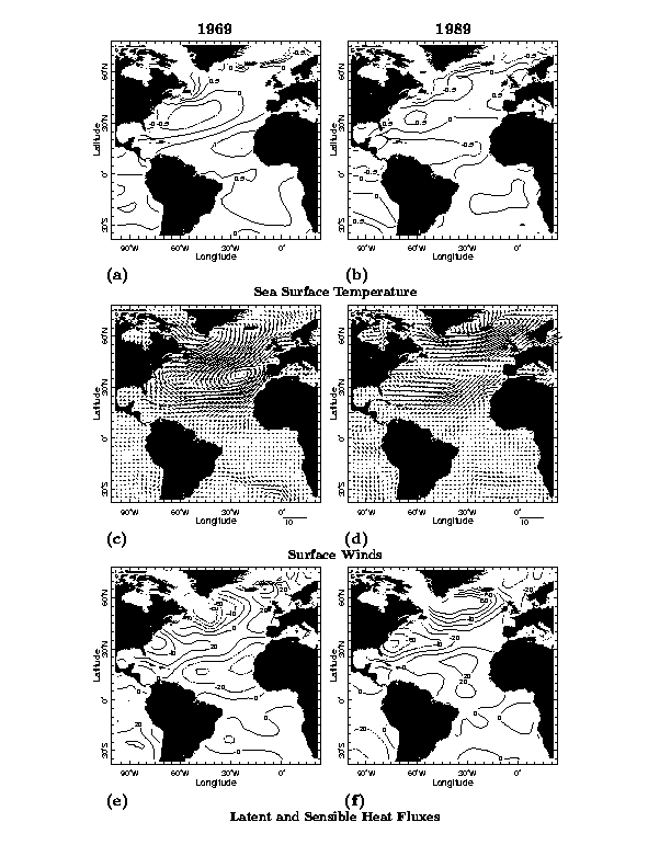
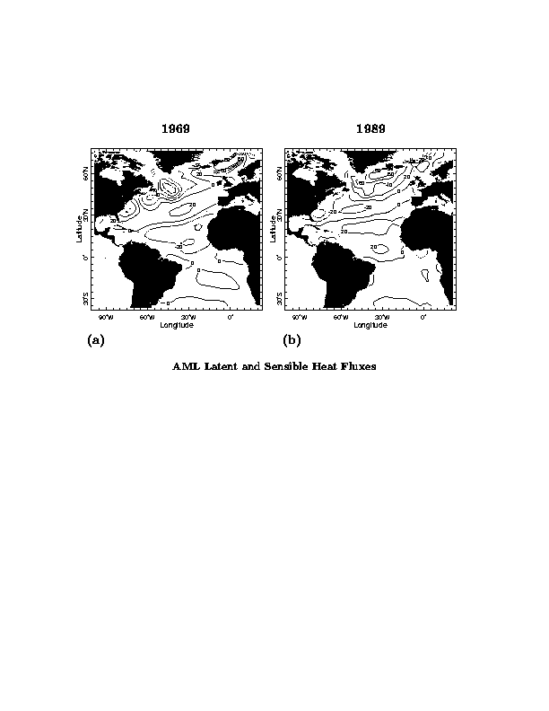
To examine the agreement between model and observed fluxes we look at two winter averages of January through March for 1969 and 1989 that exhibited opposite extreme states of the NAO. (We chose to check the model's ability to simulate the fluxes by examining specific winters, rather than an EOF for example, to emphasize that the climate variability we are talking about is clearly apparent in the raw data.) Fig. 2 shows the anomalies of SST, surface winds and upward latent plus sensible heat fluxes as derived from the NCEP reanalyses for these two winters. The latent and sensible flux anomalies are almost always the same sign. In the tropics the latent heat flux anomalies dominate, but at high latitudes they can be close to the same magnitude. Generally the anomalous turbulent fluxes are of the sign that would create the SST anomalies, e.g. anomalously positive fluxes above cold water. This relationship was noted by Cayan (1992a, 1992b) and is indicative of the atmosphere forcing the ocean. Figure 3 shows the modeled latent plus sensible heat flux when forced with observed SST. It is clear that the AML model does a reasonable job of reproducing the amplitude and spatial pattern of the observed flux anomalies.

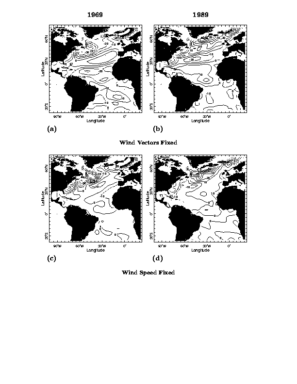
The flux anomalies could be produced by changes in wind speed or direction. Next we ran the AML model holding the wind speed and direction fixed in the advection terms but allowing the wind speed to vary in the surface flux formulation. Then we allowed the advecting winds to vary but held the wind speed in the surface flux formulation fixed. The modeled latent plus sensible fluxes for these cases are shown in Figures 4a-d. It is clear that changes in wind speed are the dominant effect south of $40^{\circ}N$, but that at higher latitudes changes in advection of temperature and moisture become important. These results are broadly consistent with the observational analyses of Cayan (1992a,1992b).