Observational analyses of atmospheric boundary layer thermodynamic budgets and SST forcing

Before attempting to model Atlantic SSTs we perform an analysis of the thermodynamic budget of the lowest part of the atmosphere. We wish to examine which terms in the budgets are responsible for the changes in surface fluxes that force changes in SST. We use the NCEP reanalyses for the period 1958-1998. We consider a layer, assumed vertically uniform, that extends from 925mb to 1000mb which we take to be representative of the atmospheric mixed layer that forms the lower portion of the boundary layer. We assume that 1000mb values are representative of the layer. Integrating from 1000 to 925 mb, and assuming a steady state on a monthly timescale, the moist static energy equation is:

$$\frac{1}{g}\left(P{\underline u} \cdot \nabla h - \omega_B(h_... ...0}{g}(h_0-h) + \frac{1}{g}(\omega''h'')_B + \frac{1}{g}c_pPR.$$ (1)

Here h is the moist static energy, $\omega_B$ is the pressure velocity at 925mb, $\omega_0=\rho C_DV$ where V is the surface wind speed and C_D is the drag coefficient, h₀ is the moist static energy of the ocean surface and h_B is that at 925mb, P is the pressure thickness of the layer (7500Pa) and R is the radiative cooling rate in Ks^-1. In this equation every term is a monthly anomaly (and includes both linear terms and nonlinear cross terms). For example the term ${\underline u} \cdot \nabla h$equals the advection evaluated for a month, using total values of u and h, minus the climatological monthly mean of that term. $\nabla \cdot ({\underline u'}h')$ is the anomalous horizontal convergence of moist static energy by eddies with timescales less than one month, $(\omega'h')_B$ is the anomalous vertical eddy moist static energy flux at 925mb. $(\omega''h'')_B$ is the anomalous vertical turbulent flux of moist static energy at 925mb. The first term on the right is the anomalous ocean to atmosphere moist static energy flux.

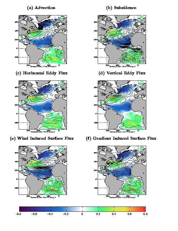
The turbulent flux and the radiative cooling rate are unknown and cannot be calculated. In the case of the radiative cooling rate this is because we are at a loss to know what the details of the cloud field were. We do not expect anomalies in the radiative cooling rate to be large but anomalies in the turbulent flux are expected to be significant. Nevertheless we are particularly interested in how changes in advection and surface and eddy fluxes impact the boundary layer temperature and humidity and, therefore, the SST. To do this we first computed EOFs of the NCEP observed SSTs. We then regressed the individual terms of the boundary layer thermodynamic budget onto the time series of the EOF expansion of SST. We only present results for the first SST mode. This mode is the familiar tripole pattern of SST anomalies that accompanies the NAO, which is virtually identical to the SST pattern emerging from the singular vector analysis discussed later, and explains 25% of the domain integrated SST variance. The figures shown are for the positive phase of the NAO when there is an anomalously strong anticyclone over the subtropical North Atlantic, a strong Icelandic low and strong mid-latitude westerlies between them. The energy budget terms, as written in Equation 1, are in Wm^-2 with the units corresponding to the flux anomaly that accompanies one standard deviation of the normalized SST anomaly time series. In the figures below the flux anomalies are contoured over the one standard deviation SST anomalies plotted in color.

The anomalous advection presents a simple pattern (Fig. 1a ). When anomalous ${\underline u} \cdot \nabla h$ is positive this represents a cooling of the boundary layer and, hence, the SST. We see that anomalous advection matches the SST pattern quite well with cool water present where there is equatorward advection in the southeastern North Atlantic and warm water present where there is poleward advection off the North American coast. Further north, anomalous flow off the cold Canadian coast and Labrador Sea area leads to cold waters offshore. The signal in the South Atlantic is weak.

Figures 1c and 1d show the horizontal and vertical eddy flux convergence. The total eddy flux convergence primarily acts to cool the warm waters east of North America. Reduced eddy fluxes warm the northern subtropics, indicative of a poleward shift of the region of maximum eddy heat and moisture fluxes. The individual eddy terms show that the horizontal fluxes almost perfectly damp the SSTs, while the vertical fluxes have maximum cooling at around $45^{\circ}N$ where the SST gradient is strengthened the most. Therefore, when summed, the cooling over, and slightly to the north of, the warm water is the dominant signal. The match between the eddy fields and the SST anomalies is quite remarkable.

The term $\omega_B(h_B-h)$, shown in Fig. 1b, represents anomalous subsidence warming and drying and is typically the same sign as $\omega$ itself. The anomalously strong anticyclone over the North Atlantic, which is also poleward of its usual position, leads to anomalous subsidence at around $35^{\circ}N$ and weaker subsidence to the south. Increased subsidence cools the SST, primarily via increased latent heat flux, by bringing down air of lower moist static energy. Changes in subsidence primarily damp the SST fluctuations.

We broke the surface flux term into two terms, the anomalous wind speed working on the mean vertical gradient of moist static energy, and the mean wind working on the anomalous vertical gradient of moist static energy. It was assumed that the nonlinear cross term was small. Figs. 1e and 1f show the regression of these terms on the SST. The flux anomaly derived from the anomalous wind speed working on the mean thermodynamic gradients perfectly matches the SST change and increases in size from pole to equator. The effects of anomalous thermodynamic gradients are more complex. In the subtropics, this gives a flux anomaly that damps the SST: increased wind speed cools the SST, and h₀ is reduced by more than h, implying that as increased surface heat loss reduces the SST the air-sea thermodynamic disequilibrium is also reduced, which tends to reduce the surface heat loss in an attempt to restore balance. North of $30^{\circ}N$ this damping effect is less obvious. In these regions anomalous advection causes anomalies in h that force SST changes.

All of these terms are of significant magnitude somewhere. Nonetheless, it is possible to draw some simple conclusions. In the subtropics wind speed changes drive changes in SST. The altered SST then creates changes in the surface fluxes that largely offset those created by the wind speed changes. North of about $25^{\circ}N$advection is important with, for the positive phase of the NAO, advection cooling the eastern Atlantic and warming the western Atlantic. Wind speed changes tend to warm the whole strip between $25^{\circ}N$ and $45^{\circ}N$. Subsidence drying also tends to cool the east. Summing these effects explains why the west warms but the SST anomalies in the east are small. Over the entire mid-latitude zonal strip atmospheric eddies primarily, and strongly, damp the SST anomalies. North of $45^{\circ}N$, anomalous advection off North America cools the SST with the reduced SST feeding back by restricting the surface heat loss. Therefore, the SST anomalies are forced by changes in the mean flow and are dissipated by transient eddy heat and moisture fluxes. This does not exclude the possibility that the changes in the mean flow are forced by changes in eddy momentum fluxes, but that will have to await further investigation.